Are you listening and reading here and there about Deep Learning and would like to have an introduction to this field?
Ok, then keep reading: in this article I will give you a very simple introduction to the basics of deep learning, regardless to the language, library or framework you may choose thereafter.
What is deep learning?
Well, trying to explain deep learning with a good level of understanding may take quite a while and it’s not the purpose of this article.
Here the purpose is to help beginners to understand the basic concepts of this field.
Nevertheless even experts may find something useful in the following content and may send me some feedback on how to improve the explanation.
At the risk of being extremely simple (you experts please forgive me) I will try to give you some basic notion. If nothing else this may just trigger the willing to study the subject more deeply for some of you.
Some History
Deep learning is essentially a new and trendy name for a subject that has been around for quite some time under the name of Neural Networks.
When I started studying (and loving) this field in the early 90s the subject was already well known in the literature. In fact, the first steps were made in the 1940s (McCulloch and Pitts [1]), but the progress in this area has been quite up-and-down since then. There were dark and bright ages, until now, when the field is having a huge success: everybody is speaking about it, deep learning is running on smartphones, cars and many other devices around us.
So, what is a neural network and what can you do with it?
Ok, let’s focus for a moment about the classical approach to computer science: the programmer designs an algorithm that, for a given input, generates an output.
He or she designs accurately all the logic of the function f(x) so that:
y = f(x)
where x and y are the input and the output respectively.
However sometimes designing f(x) may be not so easy: imagine for example that x is an image of a face and y is the name of the correspondent person. This task is so incredibly easy for a natural brain, while so difficult to be performed by a computer algorithm!
Here comes into play neural networks and deep learning. The basic principle is: stop trying to design the f() algorithm and try to mimic the brain.
Ok, so how does the brain behave? It trains itself with several, virtually infinite, pairs of (x,y) samples (the training set) and, throughout a step-by-step process, the f(x) function shapes itself automatically, not designed by someone, but just emerging from an endless trial-and-errors refining mechanism.
Think of a child watching familiar people around him or her daily: billions of snapshots, taken from different positions, perspectives, light conditions and every time making an association, every time correcting and sharpening the natural neural network underneath.
Artificial neural networks (often referred to simply as neural networks) are a model of the natural neural networks made of neurons and synapses in the brain.
Typical neural network architecture
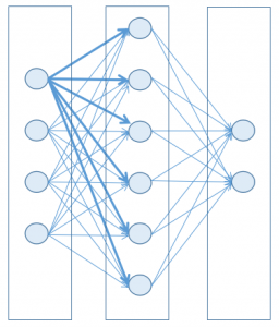
To keep things simple (and survive with the mathematics and computational power of today’s machines) a neural network may be designed as a set of layers, each one containing nodes (the artificial counterpart of a brain neuron), where each node in a layer is connected to every node in the next layer.

Each node has a state, represented by a floating number between two limits, generally 0 and 1. When this state is near to its minimum value, then the node is considered inactive (off), while when it’s near the maximum, then the node is considered active (on). You can think of it as a light bulb, not strictly tied to a binary state, but also capable of being in some intermediate value between the two limits.
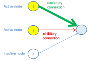
Each connection has a weight, so that an active node in the previous layer may contribute more or less to the activity of the node in the next layer (excitatory connection), while an inactive node will not propagate any contribution.
The weight of a connection may also be negative, meaning that the node in the previous layer is contributing (more or less) to the inactivity of the node in the next layer (inhibitory connection).
For the sake of simplicity, let’s describe a subset of a network where three nodes in the previous layer are connected with a node in the next layer. Again, to put it simply, let’s say the first two nodes in the previous layer are at their maximum value of activation (1), while the third is at its minimum value (0).

In the figure above the first two nodes in the previous layer are active (on) and therefore they give some contribution to the state of the node in the next layer, while the third in inactive (off) so it will not contribute in any way (independently from its connection weight).
The first node has a strong (thick), positive (green), connection weight, which means that its contribution to activation is high. The second instead has a weak (thin), negative (red), connection weight; therefore it is contributing to inhibit the connected node.
In the end we have a weighted sum of all the contributions from the incoming connected nodes from the previous layer.

where ai is the activation state of node i and wij is the connection weight that connects node i with node j.
So, given this weighed sum number, how can we tell if the node in the next layer will or will not be activated? Is the rule as simple as “if the sum is positive it will be activated, while if negative it will not”?
Well, it may be this way, but in general it depends on which Activation Function (along which threshold value) you choose for a node.
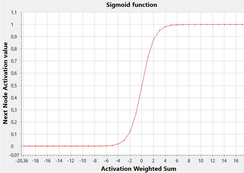
Think about it: this final number can be anything in the real numbers range, while we need to use it to set the state of a node with a more limited range (let’s say from 0 to 1). We need then to map the first range into the second, so to squish an arbitrary (negative or positive) number to a 0..1 range.
A very common activation function that performs this task is the sigmoid function

In this graph the threshold (the x value for which the y value hits the middle of the range, i.e. 0.5) is zero, but generally it may be any value (negative or positive, causing the sigmoid to be shifted to the left or to the right).
A low threshold allows a node to be activated with a lower weighted sum, while a hight threshold will determine the activation only with a high value of this sum.
This threshold value can be implemented by considering an additional dummy node in the previous layer, with a constant activation value of 1. In this case, in fact, the connection weight of this dummy node can act as the threshold value and the sum formula above can be considered inclusive of the threshold itself.
Ultimately the state of a network is represented by the set of values of all its weights (in its broad sense, inclusive of thresholds).
A given state, or set of weight values, may give bad results, that is great distance from the optimum, or a big error, while another state may instead give good results, or in other words, small errors.
So moving in the N-dimensional state space leads to small or big errors: this function, which maps the weights domain to the error value it’s the Loss Function, in the deep learning terminology. Our mind cannot easily imagine such a function in a N+1 space. However we can get a general idea for the special case where N = 2: read this article [2] and you’ll see.
Training a neural network consists, in essence, in finding a good minimum of the loss function. Why a good minimum instead of the global minimum? Well, because this function is generally not differentiable, so you can only wander around the weights domain with the help of some Gradient Descent technique and hope not to:
- make too big steps that may make you climb over a good minimum without being aware of it
- make too small steps that may make you lock in a not-so-good local minimum
Not an easy task right? That’s why this is overall the main problem with deep learning; why the training phase may take hours, days or weeks, why your hardware is crucial for this task and why you often have to stop the training and think about different approaches, different configuration parameter values … and start it all over again!
But let’s get back to the general structure of the network, which is a stack of layers: the first layer is the input (x), while the last layer is the output (y).
The layers in the middle can be zero, one or many; they are called hidden layers and the term deep in deep learning refers exactly to the fact that the network can have many hidden layers, so to become deep and therefore potentially able to find more features correlating input and output during the training.
A note: in the 1990s you would just have heard of multi-layer network instead of deep networks, but that’s the same thing. It’s just that now it became more clear that the more a layer is far from the input (deep) the more it may capture abstract features.
The learning process
At the beginning of the learning process the weights are set randomly, so a given input set in the first layer will propagate and generate a random (calculated) output. This output is then compared to the desired output for the input presented; the difference is a measure of the error of the network (loss function).
This error is then used to apply an adjustment in the connection weights that generated it and this process starts from the output layer, step-by-step backward to the first layer.
The amount of the applied adjustment can be small or big and is generally defined in a factor called learning rate.
This algorithm is called backpropagation and became popular in 1986 after a research of Rumelhart, Hinton and Williams [3].
Keep in mind the name in the middle: Geoffrey Hinton is often referred to by some as the “Godfather of Deep Learning” and he is a tireless illuminated scientist. For example now he is working on a new paradigm called Capsule Neural Networks, which sounds like another great revolution in the field!
The goal of backpropagation is to gradually reduce the overall error of the network by doing appropriate corrections to the weights at each iteration through the training set. Again consider that this process of reducing the error is the hard part, since there is not any guarantee that the weight adjustments always goes in the right direction for a good minimum.
The problem sums up into finding a minimum in a n-dimensional surface while stepping around with a blindfold: you can find a local minimun and never know if you can perform better.
If the learning rate is too small the process may result too slow and the network may stagnate in a local minimum; on the other hand a big learning rate may result in skipping the global minimum and making the algorithm diverge.
In fact quite often the problem during the training phase is that the process of reducing the error does not converge and the error grows instead of becoming lower!
Today
Why this field is having such a great success now?
Mainly because of two reasons:
1) the availablility of huge amount of data (from smartphones, devices, IoT sensors and Internet in general) needed for the training
2) the computational power of modern computers allows reducing the training phase drastically (notice that training phases of days or weeks are not so uncommon!)
Want to go deeper into the field? Here are just a couple of good books:
- Deep Learning
by Adam Gibson, Josh Patterson
O’Reilly Media, Inc. - Practical Convolutional Neural Networks
by Mohit Sewak, Md. Rezaul Karim, Pradeep Pujari
Packt Publishing
Next > Build your first neural network with Eclipse Deeplearning4j
[1] http://wwwold.ece.utep.edu/research/webfuzzy/docs/kk-thesis/kk-thesis-html/node12.html
[2] https://ml4a.github.io/ml4a/how_neural_networks_are_trained
[3] https://web.stanford.edu/class/psych209a/ReadingsByDate/02_06/PDPVolIChapter8.pdf

[…] we have seen in the first article of this series, in a classic Multi Layer Perceptron (MLP) network, each node in a layer has input […]